Interpreting Vision Models: A Conceptual Guide to Grad-CAM and Attention Maps

In the world of AI, getting a correct prediction is only half the battle. A model might correctly identify a wolf in a picture, but is it looking at the wolf, or the snow in the background? This is the core question that Explainable AI (XAI) seeks to answer. Without understanding the "why," we can't fully trust our models, debug their failures, or guard against them learning from spurious correlations.

This article moves from the theory of XAI to the practical interpretation of two of the most popular visualization methods: Grad-CAM for Convolutional Neural Networks (CNNs) and Attention Maps for Vision Transformers (ViTs). Our focus will be less on code and more on the concepts: how these heatmaps are generated, what they tell us about the model's inner workings, and how to use them as a diagnostic tool.

Visualizing CNNs with Grad-CAM

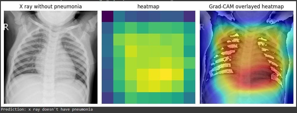
Grad-CAM (Gradient-weighted Class Activation Mapping) is a technique that produces a heatmap to show which parts of an image were most important for a model's prediction. It's like asking the model, "Which pixels made you think this was a 'cat'?"

How Grad-CAM Works: The Mechanics

The process is a clever combination of forward and backward passes through the network:

1. Forward Pass: The input image is fed through the CNN to get a final prediction. Internally, the final convolutional layer produces a set of high-level feature maps. One map might activate for "whiskers," another for "pointy ears."
2. Gradient Calculation (Backward Pass): We then take the score for our target class (e.g., 'cat') and calculate its gradient with respect to each of the feature maps from the previous step. This gradient represents how much each feature map contributed to the 'cat' prediction. A high positive gradient means that feature map was very influential.
3. Weighting the Feature Maps: The gradients are globally averaged to compute a single "weight" for each feature map. This weight signifies the importance of that map for the target class.
4. Creating the Heatmap: A weighted combination of all the feature maps is computed. This produces a coarse heatmap that highlights the regions in the image that were most responsible for the final decision. This heatmap is then resized and overlaid on the original image.

Using a high-level library like pytorch-grad-cam, this complex process is abstracted into just a few lines of code.

from pytorch_grad_cam import GradCAM
from pytorch_grad_cam.utils.image import show_cam_on_image

# model and target_layer are defined elsewhere
cam = GradCAM(model=model, target_layers=[target_layer])
grayscale_cam = cam(input_tensor=image_tensor, targets=None)

# Overlay the heatmap on the original image
visualization = show_cam_on_image(rgb_image, grayscale_cam[0,:], use_rgb=True)

What Influences a Grad-CAM Plot?

A Grad-CAM visualization is not a perfect window into the model's mind; it's an interpretation that is influenced by several factors:

• Choice of Target Layer: Applying Grad-CAM to an early convolutional layer will highlight simple features like edges and textures. Applying it to the final convolutional layer, as is standard, provides a more holistic, semantic explanation.
• Model Training and Bias: This is where Grad-CAM shines as a debugging tool. If your model was trained on a biased dataset (e.g., pictures of doctors who are all men), a Grad-CAM for the class 'doctor' might highlight a man's tie rather than a stethoscope. This reveals the model has learned a spurious correlation.
• The Target Class: Grad-CAM is class-specific. Running it for the class 'cat' will produce a different heatmap than running it for the class 'dog' on the same image containing both animals.

Using Grad-CAM to Test Robustness

By manipulating the input and observing the Grad-CAM output, you can rigorously test your model. For instance, if you show your model an image of a cow in a field, the heatmap should focus on the cow. If you then show it an image of a cow on a beach and the heatmap shifts to the water, your model is not robust and has likely overfitted to "cows are in grassy fields."

Visualizing Vision Transformers with Attention Maps

Vision Transformers (ViTs) have a built-in mechanism for explainability: the self-attention scores. These scores determine how much each image patch "attends to" or focuses on every other patch when forming its representation.

How Attention Maps Are Generated

1. Image Patching: A ViT first splits an image into a grid of patches (e.g., a 224x224 image becomes a 14x14 grid of 16x16 patches).
2. The [CLS] Token: A special, learnable [CLS] (classification) token is added to the sequence of patch embeddings. This token's job is to aggregate information from all patches to make the final prediction.
3. Visualizing Attention: After the model is trained, we can inspect the attention scores from the final layer. Specifically, we look at the attention from the [CLS] token to all the image patch tokens. A high score indicates that a patch was highly influential in the final decision.
4. Creating the Heatmap: These attention scores are reshaped into a 2D grid (e.g., 14x14) and then resized to the original image dimensions, creating a heatmap that shows the model's focus areas.

A simplified code representation would look like this:

# Assume a helper function gets the attention from the last layer
attention_scores = get_last_attention_from_model(vit_model, image_tensor)

# Get attention from the [CLS] token and average across heads
cls_attention = attention_scores[0, :, 0, 1:].mean(dim=0)
heatmap = cls_attention.reshape(14, 14) # Reshape to patch grid

# Now, resize and plot the heatmap over the image
plt.imshow(heatmap.cpu().numpy(), cmap='jet', alpha=0.5)

What Influences an Attention Map?

• Layer Depth: Attention maps from the initial layers of a ViT are often broad and diffuse, as the model is gathering global context. Maps from the final layers are much sharper and more focused on the semantically important objects.
• Attention Heads: A ViT has multiple "attention heads," and each can learn to focus on different aspects. Some heads might learn to find outlines, others textures, and others might focus on contextual objects. Averaging them provides a general explanation, but analyzing them individually can offer deeper insights.

Using Attention Maps to Test Robustness

Attention maps are excellent for understanding a model's failure modes. If a model misclassifies an image, the attention map can reveal whether it was "distracted" by an irrelevant object in the background. You can also perform occlusion experiments: by blacking out the area where the model is focusing, you can test if it's robust enough to find the object in other parts of the image or if its understanding is brittle.

Conclusion

Grad-CAM and Attention Maps are more than just pretty pictures; they are powerful diagnostic tools. They allow us to move beyond measuring if a model is correct and start asking why. By using them to probe our models, we can uncover hidden biases, diagnose failures, and build more robust, trustworthy, and reliable AI systems.

Enjoyed this post? Subscribe to the Newsletter for more deep dives into ML infrastructure, interpretibility, and applied AI engineering or check out other posts at Deeper Thoughts