When GANs get Convincing (and when they Collapse): The Art of Faking It till you Make it

Generative Adversarial Networks (GANs) have emerged as a powerful framework for modeling complex, high-dimensional data distributions without relying on explicit density estimation. Their ability to generate photorealistic images, translate styles across domains, synthesize data for augmentation, and contribute to scientific discovery such as molecular design, positions GANs at the forefront of generative modeling research. These models excel in capturing intricate data structures, producing samples that often rival real-world data in fidelity and diversity.

However, the intricate dynamics of their training processes, including issues like mode collapse and instability, present ongoing challenges that require sophisticated techniques and deeper theoretical insights. As GANs continue to push boundaries in both practical applications and fundamental research, what underlying principles govern their generative capabilities, and how can we further improve their robustness and versatility across such diverse fields?

• GAN 101: The Foundations of Generative Modeling
• GAN Training Paradigm - A Mathematical glance
  • Generator (G)
  • Discriminator (D)
  • What Makes This Paradigm Unique?
• Evaluating GANs : How do we improve them over epochs
• What GANs learn: Representation and Feature Disentanglement
• Failure Modes: When GANs Don’t Make It
• Advances to Mitigate Failures
• Conclusion

GAN 101: The Foundations of Generative Modeling

Imagine trying to teach a machine to paint – not by telling it exactly how a painting should look, but by asking it to fool an art critic. That’s the central idea behind Generative Adversarial Networks (GANs).

At a high level, generative models are algorithms that learn to create new data similar to what they've seen before — like generating realistic-looking images, audio, or even text. There are many families of such models:

• Autoregressive models like PixelRNN or PixelCNN build images one pixel at a time, modeling each pixel based on the ones before it. They're accurate but very slow to sample from.

• Variational Autoencoders (VAEs) learn a compressed code of the input and decode it back to an image. They’re stable and interpretable, but often produce blurry outputs because they optimize pixel-wise reconstruction.

• Diffusion models such as Stable DIffusion start with pure noise and learn to denoise it step-by-step until an image emerges. They generate stunning results but are computationally expensive and slow to sample from.

GANs, on the other hand, take a completely different approach. They don’t bother modeling the exact probability of your data. Instead, they train two networks simultaneously: The generator improves by learning how to produce images that are increasingly difficult to distinguish from real ones. The discriminator improves by getting better at catching the fakes.

This dynamic training process is what gives GANs their edge: they can produce sharp, detailed, and incredibly realistic images, often better than VAEs or autoregressive models. But it’s also what makes them notoriously difficult to train. Problems like mode collapse (where the generator produces the same output repeatedly) or unstable feedback loops are common.

GAN Training Paradigm - A Mathematical glance

A GAN essentially has two major components

Generator (G)

• Takes random noise z (often Gaussian or uniform) and maps it to the data space to produce a fake sample G(z).
• Goal: Fool the discriminator into thinking fake samples are real.

Discriminator (D)

• Takes in either real data x or generated samples G(z), and outputs a probability that the input is real.
• Goal: Correctly classify real vs. fake.

The networks are trained simultaneously, with opposing objectives. In practice, a value function V is calculated during each step of training.

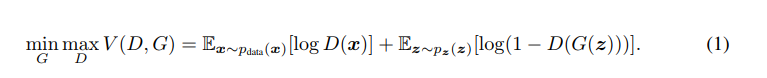
• Discriminator D wants to maximize this function — get better at telling real from fake.
• Generator G wants to minimize it — produce samples that fool D.

  In practice, instead of minimizing log(1 - D(G(z))), which can lead to vanishing gradients when D(G(z)) ≈ 0, we often maximize log(D(G(z))). This alternative is called the non-saturating loss and provides stronger gradients early in training, helping the generator learn faster.

What Makes This Paradigm Unique?

• No direct supervision: Unlike classification, GANs don’t require paired input/output labels.
• Adversarial feedback: The generator improves solely from the discriminator’s judgment.
• Unstable equilibrium: The networks are optimizing against each other, not a fixed objective.

In simpler terms, The generator creates a batch of fake images from random noise. The discriminator then evaluates these along with real images, outputting real/fake labels. Both networks are updated via backpropagation: the discriminator learns from the true labels, and the generator receives gradients aimed at increasing the discriminator’s error. This loop repeats, so over time the generator’s outputs steadily improve and the discriminator must adapt to distinguish the more realistic fakes.

Evaluating GANs : How do we improve them over epochs

Unlike supervised learning, GANs lack a straightforward metric like classification accuracy. Researchers typically use proxy metrics that correlate with image quality and diversity. One of the most common metrics researchers and engineers use to evaluate their GANs is the Inception Score (IS). IS is an entropy based metric that uses a pretrained image classifier (Inception network) on generated samples. A good model should produce images that the classifier recognizes confidently (low entropy of predicted label) and with overall diversity (high entropy of predicted label distribution).

More recent work argues that single-number metrics hide important information. Precision measures fidelity (are generated samples realistic?) and recall measures coverage (do we produce all modes of the data?). Empirically, GANs tend to have high precision but low recall (they create very sharp images but miss modes, e.g. only generate a subset of digit classes). whereas VAEs have higher recall (cover modes) but lower precision (blurrier samples).

Qualitative assessment (visual inspection of samples) remains important. Overfitting checks are also used: for example, comparing generated samples to nearest neighbors in the training set. If a GAN simply memorizes training images (an extreme overfit), generated examples will look identical to real ones.

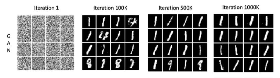
In practice, watching the training loss curves can give clues: if D loss goes to zero and G loss explodes, D may be overpowering G. Ideally, over epochs D stays around 50% accuracy (it can’t distinguish real/fake much better than chance) while G steadily improves sample quality. But what are these GAN's then really learning?

What GANs learn: Representation and Feature Disentanglement

One of the most fascinating properties of GANs lies in what they implicitly learn about the structure of the data distribution — often without any labels or explicit supervision. This becomes particularly evident when we explore the latent space in which the generator operates. Linearly interpolating between two such latent vectors results in a smooth and semantically meaningful morph between generated images. For instance, interpolating between two vectors that generate images of different faces may produce a series of intermediate faces that gradually blend one into the other — changing age, expression, pose, or even lighting in a coherent and gradual fashion.

This phenomenon implies that the latent space has learned a smooth, meaningful manifold — one where proximity in the latent space reflects semantic similarity in the output space. This wouldn't happen if the generator simply memorized images.

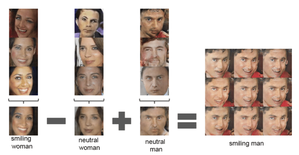
Even more intriguingly, in many GAN variants (particularly those trained with regularization or architectural tweaks like InfoGAN or StyleGAN), the latent space exhibits disentanglement — meaning different dimensions of z control different semantic attributes of the output. One direction may change hair color, another might rotate the object, and yet another might add eyeglasses or a smile. These interpretable transformations suggest that GANs are learning internal representations that separate out the independent factors of variation in the data — a long-standing goal in representation learning.

These properties hint at the potential of GANs for controllable and interpretable generation, with use cases in image editing, data augmentation, and unsupervised representation learning. For example, in medical imaging, a disentangled GAN can be used to synthesize new patient images with varied pathologies while keeping anatomical structures fixed. In design, one could traverse the latent space to explore fashion or architecture variations.

But this raises a deeper question: If GANs can learn such rich, structured representations — why do they sometimes fail so catastrophically?

Failure Modes: When GANs Don’t Make It

While GANs have unlocked jaw-dropping capabilities in image synthesis, style transfer, and beyond, they’re walking a tightrope behind the scenes. Two neural networks locked in a game of deception can produce magic — but only if their rivalry stays perfectly balanced. Tip the scales even slightly, and things can go haywire. These condiitons are what we call failure modes.

So, what exactly goes wrong when GANs fail? And why does it happen so often? Let’s dig into the most common failure modes that plague GANs — and why understanding them is key to building truly reliable and optimized generative models.

• Mode collapse: The generator ignores parts of the data distribution and produces only a few outputs (sometimes even the same output repeatedly). For example, a GAN on digit images might only generate “6”s and “9”s. This happens when Generator G finds a small set of samples that consistently fool the Discriminator D, and has no incentive to explore other modes. The result is low diversity (low recall). Empirically, GANs often exhibit partial collapse where several distinct samples map to nearly identical outputs. This issue was already noted in the original GAN literature

• Vanishing or exploding gradients: If the discriminator becomes too confident (e.g. perfectly separating real and fake), the generator’s gradient (∇G) can vanish to zero. Then G stops learning. Conversely, unstable training can cause gradient explosions, saturating activations (e.g. outputs saturating at 0/1).

• Non-convergence and oscillation: GAN training is not guaranteed to converge to an equilibrium. Instead, G and D may keep chasing each other in a loop. For instance, G produces more realistic fakes, then D recovers and discerns them, then G adapts, etc. In practice, the losses may oscillate or ping-pong without settling. This can be seen as fluctuating PSNR over epochs.

These failures often go hand-in-hand: for example, mode collapse is partly caused by vanishing gradients to other modes. In practice, one sees a “chain of doom”: D becomes very good, then G collapses, then D quickly re-learns to reject whatever G produces, and training diverges. Diagnosing these failures usually involves inspecting generated samples and losses. For instance, if D’s loss quickly goes to zero and G loss stops improving, one might have found catastrophic failure. On simpler datasets (e.g. MNIST), visualizing generated digits can immediately reveal mode-dropping.

Advances to Mitigate Failures

Much progress has been made to improve GAN stability and performance. The Wasserstein GAN (WGAN) was introduced with the idea of penalizing the gradient norm of D on interpolated samples. This largely eliminated problems caused by weight clipping and is now standard for stabilizing GANs. Other techniques aim to address mode collapse by forcing the generator to produce variation. Minibatch discrimination lets D look at relationships between samples in a batch, penalizing lack of diversity. Feature matching trains G to match statistics (like mean activations) of real vs. fake batches. Both encourage the Generator to cover more modes rather than collapsing.

Studies have also found that different learning rates for G and D can help reach an equilibrium where both networks improve together; for example, D might use a larger learning rate.

Incorporating self-attention or residual blocks has also shown to help D evaluate global context and G coordinate structure across the image. Advanced GAN architectures like SAGAN use Self-Attention to to allow both the generator and discriminator to model long-range dependencies and integrate features from spatially distant regionswithin the image. This is particularly useful in generating globally coherent structures — for example, ensuring that both eyes in a face align or that symmetrical patterns in objects are preserved.

(To understand how attention mechanisms shape generative models, check out my detailed blog post on self-attention in generative networks [Link] )

Conclusion

Generative Adversarial Networks have pushed the boundaries of synthetic media, enabling realistic image synthesis, style transfer, data augmentation, and even super-resolution — applications that span creative industries to scientific domains. But as GANs become more powerful, they also tread into ethically complex terrain. From fabricated celebrity deepfake videos circulating on social media, to AI-generated humans indistinguishable from real ones, to synthetic datasets used without clear provenance — the line between creative potential and misuse grows thinner. These challenges are not flaws of the architecture, but of deployment without guardrails.

As GANs continue to evolve with more stable, expressive, and controllable designs, so must our frameworks for transparency, attribution, and responsible use. After all, in a world where machines can convincingly fabricate reality, identifying what is real becomes just as valuable as innovating to get as real as possible.